
Introduction
In this blog post I will explain how to write a simple ray marcher in CUDA hopefully without making it too technical… At least I’ll try my best. The post is divided into three parts. First, we’ll look at how the ray marching process works and what signed distance functions are. After that, we will have a quick introduction to CUDA. We will of course avoid the advanced and scary stuff because, frankly, I don’t know most of it either. Fortunately, it doesn’t prevent us from making something that can create pictures though! In the last section we will look at how I implemented everything in one of my personal projects. The reason I wrote a ray marcher was that I wanted to create fractals based on SDF formulas that were available online, but as far as I know there’s no way to access rays while Houdini is rendering. I also thought it would be a good idea to learn more about CUDA.
The code for my ray marcher is on GitHub: https://github.com/jonathangranskog/simpleCudaRayMarcher/
Basics of Ray Marching
So let’s get right into it. Before we can start talking about anything else, let’s first understand what an SDF is. SDFs is the abbreviation of signed-distance field or signed-distance function, both are commonly used. The name sounds fancy and technical, but actually it is pretty clear. ‘Function’ or ‘Field’ suggests that at some (3D) point you can get a value. What is the value you ask? Well, it’s just a distance to the nearest surface. And ‘signed’ simply means that the distance uses plus and minus signs to describe whether the point is outside or inside the surface. A positive value X returned from an SDF at some point in space means that the point is outside the surface and if you move X units in some direction you will be on the surface of some object. Negative values means that the point is inside the object and similarly if you move X (without the minus sign) units you will be on the surface. That’s really all there is to SDFs.
Then, what does the name ‘Ray Marching’ mean? Well maybe you’ve heard of ray tracing, which is used in most offline rendering nowadays. In ray tracing you intersect rays with objects in a scene to find the closest surface in a certain direction starting from a certain point. In ray marching, instead of finding intersections based on geometric formulas, you march through the scene in a certain direction from a starting point until you come close enough to something that you can consider it a hit. And how do you know the distance to a surface? SDFs, surprise surprise! In short, the difference between ray tracing and marching is just the way the scene is described. Ray tracing uses geometric primitives (triangles mostly) while in ray marching we have SDFs.
So how do you march through the scene? You start at the starting point and then you take steps in a given direction. At every step you add the direction multiplied by some constant to the previous 3D point and then you evaluate the SDF to see if you are close enough. You could always use the same constant to multiply the direction to take even steps, but that would be pretty stupid considering we know thanks to the SDF how far away the nearest surface is. So instead, we can use the distance from the SDF to multiply the direction. And then when we are close enough to a surface we stop marching and return some information about what we hit. However, an important thing to keep in mind is that the nearest surface might not be in the direction we are going. It’s not perfect, but it’s definitely better than taking constant steps.

Now, as you might already know, surface normals are necessary for shading in computer graphics. Scalar fields (SDFs are scalar fields) have a property called the gradient, which is a vector pointing in the direction of the biggest change from any point. The gradient also turns out to be the normal of a surface. So all we need to do is evaluate the gradient at the hit point to get the normal. To evaluate the gradient, we need to calculate the derivative at our point. Now this might sound complicated, but really what we do is we take a tiny step along each of our 3D axis vectors in both positive and negative directions and then we evaluate the SDF in each of these points. Based on the differences between the positive and negative direction values we will know along which axis the values changed the most. By normalizing the result we get the normal.
fx = SDF(point + (step, 0, 0)) - SDF(point - (step, 0, 0))
fy = SDF(point + (0, step, 0)) - SDF(point - (0, step, 0))
fz = SDF(point + (0, 0, step)) - SDF(point - (0, 0, step))
normal = normalize(fx, fy, fz)
This is really all you need to understand about ray marchers. In the last part you can see how I’ve implemented all of this. But before we can look at my implementation, we need to cover some CUDA concepts.
A Short Introduction to CUDA
A GPU is a component in your computer that is very good at running independent processes in parallel. And because we have multiple pixels whose results are independent of each other GPUs work really well in rendering. One way to program for GPUs is to use CUDA. CUDA’s syntax is similar to C++ so it’s fairly easy to get started with but unfortunately it only works on NVIDIA’s GPUs (because NVIDIA created it, duh).
Let’s go through some terms. In CUDA the GPU is called ‘Device’ and the CPU is called the ‘Host’. The host and the device don’t share memory so when you have some data on the CPU that you want to process on the GPU you have to move it over. CUDA has a function that allocates memory on the GPU (cudaMalloc) and in CUDA you can also copy memory from one to the other (cudaMemcpy). When you don’t need the memory you’ve allocated you need to free it (cudaFree). In CUDA you can write functions for the GPU and/or the CPU, so functions need to specify for which component they are supposed to run on. This is done by adding __device__ or __host__ in the function definition. You can also put both after each other which means that the function can run on both the CPU and the GPU.
There’s another function which is called for each thread and is used to start a process on the GPU. This is called the ‘Kernel’. It is the main function in a CUDA program. The kernel is run for each thread and from the kernel you can call __device__ functions, but not __host__ functions. Instead of __device__, a kernel function is defined with __global__ and when you call a kernel you also need to specify how many GPU threads will run the kernel. We will see an example in the code later.
Two more things left to mention before we can look at my implementation. In CUDA, 3D vectors are of type float3 and you create one using the make_float3() function. Random values are a little bit trickier in CUDA than on the CPU. For each thread you need to initialize a random state based on a seed. The random state object type is called curandState and it is initialized with a seed using a function called curand_init(). Then when you want the next (uniform) random value you have to call another function, which is called curand_uniform(). When managing a curandState you will have to pass the state’s pointer around because it is given as input to the curand functions. Don’t worry if this feels a little confusing, hopefully looking at the code will make everything a tiny bit clearer.
Implementation Walkthrough

The main function is where the CPU execution starts. It creates all the necessary variables we need for the kernel function. First it defines the width and height of the image. Then the amount of threads used for the kernel. Here each block is square and contains block size squared number of threads. The number of blocks is based on the dimensions of the final image.
The next part simply creates a camera with some data about where it’s looking and its field of view.
After the camera definition, there’s a for loop that calls the render kernel on each iteration. The input that changes is the t value going from 0 to 1 based on which frame we are. By using this t value in the SDFs we have a simple way to create some animation. You can also see that there’s some memory management going on in the loop. Basically all that happens is that we allocate an image on the GPU, which has RGBA (4 components) for each pixel, and when we render the results are stored in the GPU image. When the kernel is finished, the GPU image is copied into CPU memory and then saved as a .png using lodepng (saveImage). After the image is saved on the disk we free both CPU and GPU memory and move on to the next iteration.
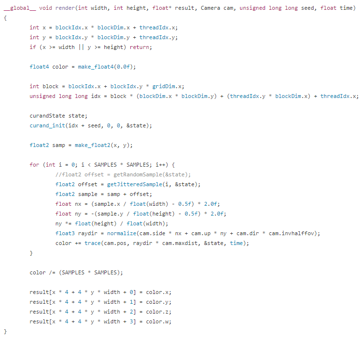
As you saw, the program calls the kernel on each iteration. The kernel then runs on the GPU to get some color value which is stored in the image. The first few rows of the kernel calculates an indices for the thread and sees if it’s inside the image. If not, we quit execution on the current thread. Note, this doesn’t quit execution for all threads. Only for the current one. The others keep chugging along happily until they are finished. The next part defines a seed for the random state and initializes it using curand_init().
If you are familiar with computer graphics at all, you might have some idea of what the for loop does. Instead of firing a single ray through the center of a pixel, we want to take many samples through the same pixel to remove as much noise as possible. This is done by summing up multiple samples through various points in the pixel and averaging the results. The curandState is passed into getJitteredSample() that returns a random 2D sample between [0, 1] in x and y. This is then added to the pixel coordinates of the current pixel in the image.
The final sample coordinates of the image now needs to be transformed so we get a ray direction that points from the camera position to the sample position on the camera plane. The sample coordinates are still in image coordinates, meaning for a 1080p image the x coordinate goes from 0 to 1920 and the y coordinate from 0 to 1080. What we really need is values that go between [-1, 1] where (0,0) is the center of the image plane. This is what nx and ny calculate. We know that nx and ny go from -1 to 1 and now based on the field of view we calculate how far away the image plane is from the camera. Then combining nx, ny and image plane distance with the camera’s vectors we get the final ray direction to march along.

How to get the ray direction
As you can see in the code, the trace function is called from render but let’s ignore it for a moment. Let’s just assume that instead we call march and take its hit.color instead as the result. The trace function does some basic path tracing, which we won’t get into just yet.

So, how does marching work? As you can see it’s a device function that returns a Hit object. Basically it does exactly what was described in the ray marching section of this post. It starts at the camera origin and moves along our ray direction with step sizes based on the nearest distance. DE is a function that returns the “distance estimation”, which is the signed-distance really. The while loop keeps running until we either hit something or move too far away in space that we can assume that we won’t hit anything anymore. When we are at a point where the distance is less than MINDIST we decide that the point is on a surface and then we calculate the normal as previously described. Finally we return all the hit information.

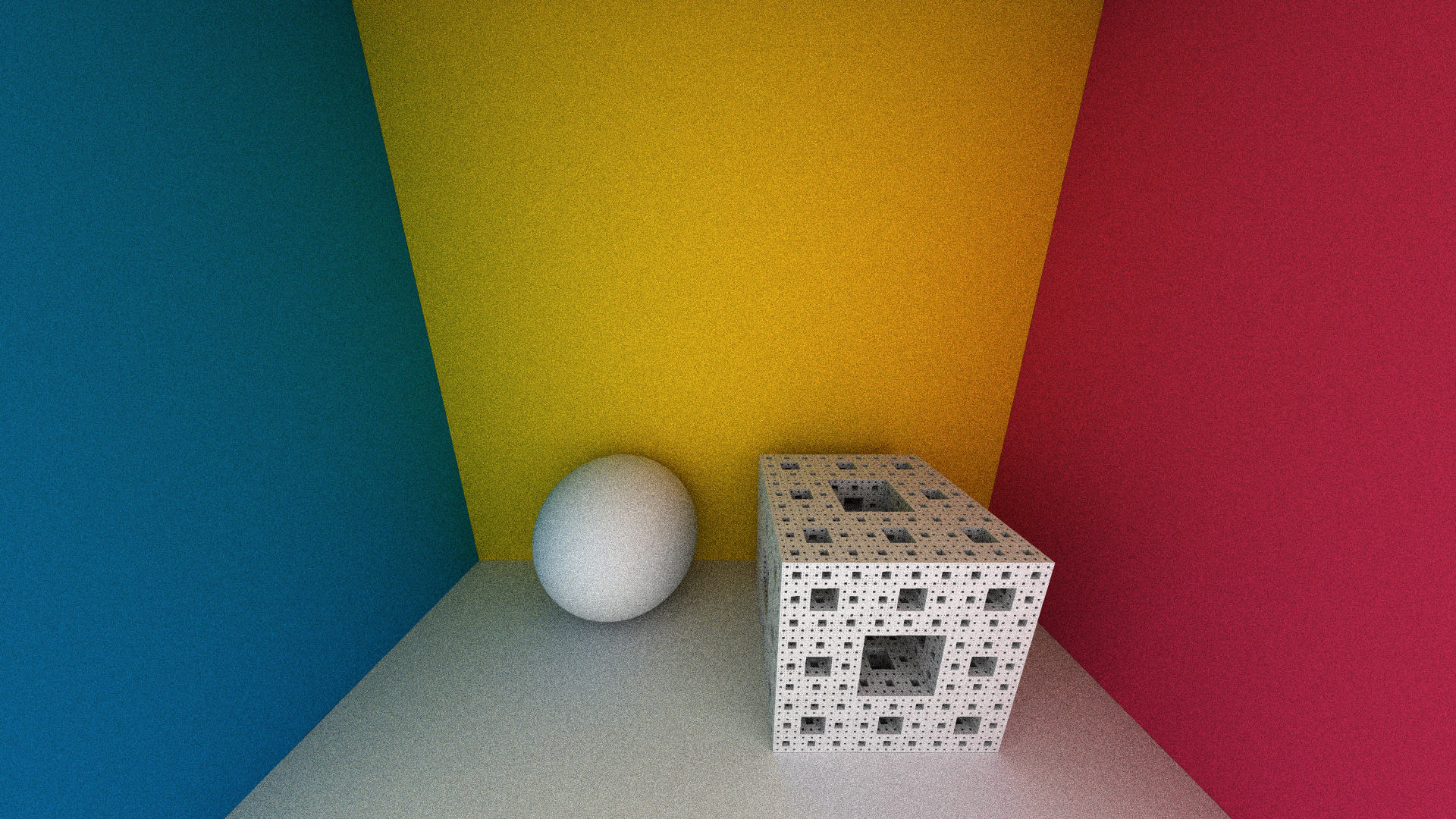
So to get prettier pictures I decided to implement basic path tracing, which means only diffuse and no lights. Everything is surrounded by a big gray sphere that lights everything evenly. This creates an ambient occlusion look. In short, path tracing is used to simulate global illumination by following rays around in a scene when they bounce and collect light. The loop in the trace function collects hit colors in the mask vector until the ray flies out and hits the big gray sphere. If it doesn’t it means that the path was never got any light and the color is not visible. Everything that doesn’t hit an SDF surface is assumed to hit the glorious surrounding sphere, unless it’s the first ray then we set the alpha component to 0 to give us transparency in the final image.
Everything here is also physically based because the orient function that creates the next ray direction is generating a cosine-distributed vector in the hemisphere which cancels out the pdf division (sorry, this is a little more advanced and not something I will go into here).
The SDFs are mostly based on other people’s work and I have just collected a bunch of formulas together into one project.
http://www.fractalforums.com/sierpinski-gasket/kaleidoscopic-(escape-time-ifs)
http://www.iquilezles.org/www/articles/distfunctions/distfunctions.htm
http://blog.hvidtfeldts.net/index.php/2011/06/distance-estimated-3d-fractals-part-i/
References
Inigo Quilez www.iquilezles.org
Fractal Forums: http://www.fractalforums.com/
Syntopia http://blog.hvidtfeldts.net/
CUDA docs http://docs.nvidia.com/cuda/
Ray Tracey https://raytracey.blogspot.fi/2015/10/gpu-path-tracing-tutorial-1-drawing.html